Norton's Theorem as a Fairy Tale: A Spring, a Hidden Aqueduct, Two Formulas, and Six Caveats

The previous article used the "black-box castle" to explain Thévenin's theorem (see Explaining Thévenin's Theorem with a Black-Box Castle); this one completes its parallel sibling: Norton's theorem.

Why learn another one? Because Thévenin is "a voltage source in series with a resistor," naturally suited to series voltage division, ADC sampling, and cascaded amplification. But many real board structures are parallel—multiple supplies tied together, a pile of branches hanging off the same node, a constant-current source driving an LED, a 4–20 mA current loop. In those cases Norton lets you write the node equation in one line, whereas Thévenin forces you to do source transformations back and forth.

The Story: A Spring and a Hidden Aqueduct

Same black-box castle in Mist Valley, same little fox Ali, same two copper nails on the wall. But this time Ali isn't fetching water in a bucket—it needs to drive a water mill, so it cares not about how high the water level is, but how strong the flow is.

Grandpa Copper Nail says: last lesson you asked "how high is the water pressure at the door," this lesson asks "how strong is the water flow at the door." Same castle, two questions—and therefore two sets of incantations.

Incantation One: Connect the Terminals with a Zero-Resistance Pipe

Take a short, fat, completely effortless pipe and connect the two copper nails (short circuit)—water gushes out at the maximum flow it can deliver. Measure it with a flow meter, and that number is the Norton current:

$$I_N = I_{sc}$$

Why? Because there's no external resistance at all, so every "self-dispensing" source inside the castle pushes out its full share. That's the definition of short-circuit current.

⚠️ In reality, never actually short a supply with a wire (see Caveat 1 at the end). What we're measuring here is an idealized operation—in engineering, we calculate it.

Incantation Two: Put the Castle's Magic Sources to Sleep

This step is exactly the same as in the Thévenin lesson: short voltage sources, open current sources (controlled sources stay put), and the equivalent resistance measured looking out from the two copper nails is the Norton resistance:

$$R_N = R_{th} = \frac{V_{oc}}{I_{sc}}$$

For the same black box, the Thévenin resistance and the Norton resistance are the same number. That's no coincidence—the transformation formulas later will explain why.

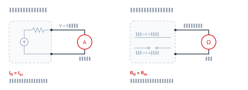
Figure 1: The physical version of the two incantations. Left: "zero resistance at the outlet—measure the maximum flow." Right: "put the magic sources to sleep—measure how rough the pipe is." Note that $R_N$ and $R_{th}$ are the same number.

Incantation Three: Fold It into "One Spring + One Aqueduct"

$$\boxed{\;\text{Any linear two-terminal network} \;\equiv\; I_N \text{ in parallel with } R_N\;}$$

In water terms: inside the castle there's effectively a spring that gushes $I_N$ at a constant rate every second, plus an internal hidden aqueduct $R_N$ through which water can loop back inside the castle without ever coming out.

Once you connect your water wheel $R_L$, the spring's water splits between two paths:

$$I_L = I_N\cdot\frac{R_N}{R_N+R_L},\qquad V_L = I_N\cdot\frac{R_N R_L}{R_N+R_L}$$

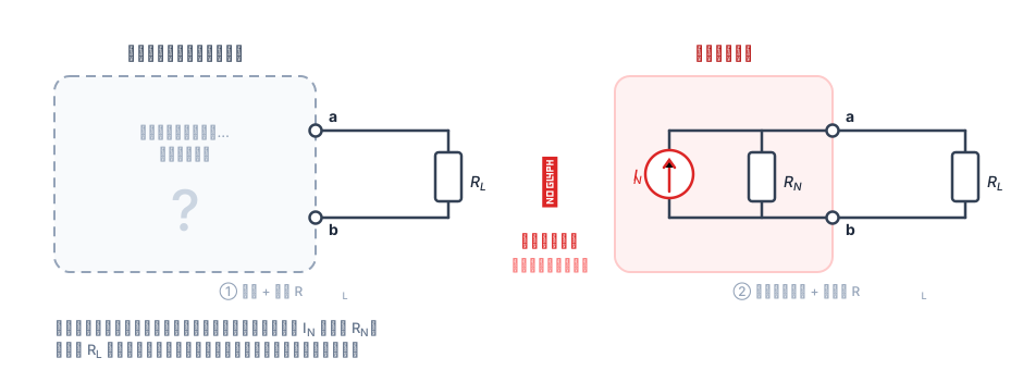
Figure 2: The load $R_L$ is drawn outside the box—only what's inside the box gets transformed. To the outside, the whole castle equals "a constant-current spring $I_N$ in parallel with a hidden aqueduct $R_N$"; the same $R_L$ behaves identically on either side.

That's parallel current division. The lower-resistance path takes most of the water:

• $R_L \ll R_N$ (your pipe is short and fat) → $I_L \to I_N$: almost all of it goes to you;
• $R_L = R_N$ (both paths equally rough) → $I_L = I_N/2$: the water splits exactly in half;
• $R_L \gg R_N$ (your pipe is pathetically thin) → almost all the water escapes through the hidden aqueduct, but now $V_L \to I_N R_N$, which is the open-circuit voltage.

That last one is worth remembering: the Norton model already carries all of Thévenin's information—the open-circuit voltage is simply $I_N \times R_N$.

Trial: The Same 12 V Voltage-Divider Castle

Use the same castle from the previous article for comparison: a $12\,\mathrm{V}$ supply in series with $R_1 = 6\,\mathrm{k\Omega}$, then $R_2 = 3\,\mathrm{k\Omega}$ to ground, with the port taken across $R_2$.

Short-circuit current (short a and b directly; now $R_2$ is bypassed and the supply sees only $R_1$):

$$I_{sc} = \frac{12\,\mathrm{V}}{6\,\mathrm{k\Omega}} = 2\ \mathrm{mA} = I_N$$

Lights-out resistance (short the 12 V source, $R_1 \parallel R_2$):

$$R_N = 6\,\mathrm{k} \parallel 3\,\mathrm{k} = 2\ \mathrm{k\Omega}$$

Connect a $2\,\mathrm{k\Omega}$ water wheel (exactly as rough as the hidden aqueduct, so it splits in half):

$$I_L = 2\,\mathrm{mA}\times\frac{2}{2+2} = 1\ \mathrm{mA},\qquad V_L = 1\,\mathrm{mA}\times 2\,\mathrm{k\Omega} = 2\ \mathrm{V}$$

Exactly matches the 2 V / 1 mA from the Thévenin lesson—two paths, one answer.

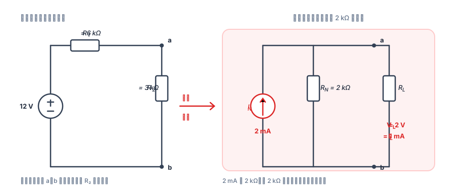
Figure 3: $I_N = 12\,\mathrm{V}/6\,\mathrm{k}\Omega = 2\,\mathrm{mA}$, $R_N = 6\,\mathrm{k}\parallel 3\,\mathrm{k} = 2\,\mathrm{k}\Omega$; the load is also $2\,\mathrm{k}\Omega$, both paths are equally rough, and the current splits exactly in half.

When to Use Norton: Watch for "Parallel" vs. "Series"

	Thévenin ($V_{th}$ in series with $R_{th}$)	Norton ($I_N$ in parallel with $R_N$)
Best suited for	Series voltage division, cascading, ADC sampling impedance	Parallel supplies, node analysis, constant-current drive
Equation form	Loop / KVL direct substitution	Node / KCL direct substitution (one branch per term)
Parameters from	$V_{oc}$ + lights-out method	$I_{sc}$ + lights-out method
No load	$V = V_{th}$	$V = I_N R_N$
Short circuit	$I = V_{th}/R_{th}$	$I = I_N$

The two can be interchanged at any time; the conversion is just a source transformation:

$$I_N = \frac{V_{th}}{R_{th}},\qquad V_{th} = I_N R_N,\qquad R_N = R_{th}$$

Don't memorize it as something new: Norton's theorem = Thévenin's theorem + one source transformation. The reverse is also true, so when you see an exam problem like "replace a voltage source in series with a resistor by a current source in parallel with a resistor," you're essentially applying Norton.

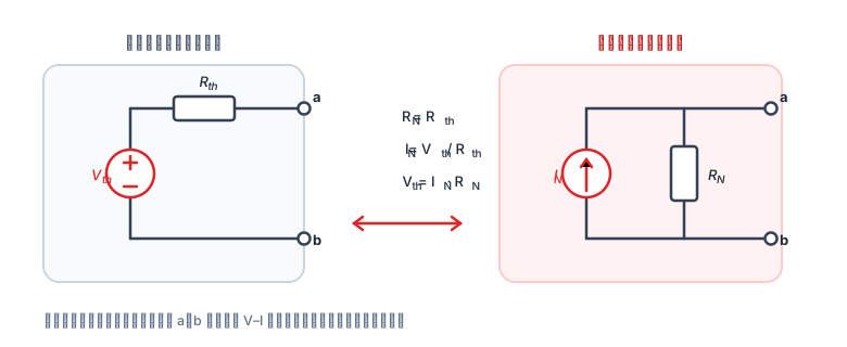
Figure 4: Two ways of writing the same $V$–$I$ line. These three rows are all you need: $R_N = R_{th}$, $I_N = V_{th}/R_{th}$, $V_{th} = I_N R_N$.

Six Caveats (All the Pitfalls I've Stepped In)

1. Don't Actually Short the Output Just to Measure $I_{sc}$

Short-circuit current is an idealized parameter. The instant you short a real supply, the current can be tens of amps: at best it sags the rail and trips overcurrent protection, at worst it blows transistors and burns traces. The safe approach is to measure the open-circuit voltage, compute the internal resistance with the lights-out method, and back-calculate:

$$I_N = \frac{V_{oc}}{R_{th}}$$

If you really must measure it, insert a current-limiting resistor or use an electronic load, measure at a small current, and extrapolate linearly.

2. It's Only Valid for the Port—Never Use It for Internal Power

This is the same pitfall as in the Thévenin lesson, and Norton is no different. Take the same 12 V divider above with a $2\,\mathrm{k\Omega}$ load:

	Supply output	Load receives	Internal loss
Real circuit	$12\,\mathrm{V}\times1.667\,\mathrm{mA}=20\,\mathrm{mW}$	$2\,\mathrm{mW}$	$R_1$ 16.7 mW + $R_2$ 3 mW = 19.7 mW
Norton equivalent	$I_N \times V_L = 4\,\mathrm{mW}$	$2\,\mathrm{mW}$	$R_N$ (1 mA) 2 mW

The port voltage and current are identical, but the internal loss differs by almost ten times. The equivalent circuit is only a stand-in at the door—using it to calculate efficiency, resistor power, or temperature rise will all be wrong.

3. The Current-Source Direction Is the Easiest to Get Backwards

The arrow on $I_N$ = the direction the short-circuit current actually flows (out of the terminal marked "+"). Get the direction backwards and every voltage sign downstream flips. After drawing a Norton circuit, double-check one thing: if you short a and b, does the current flow in the direction of the arrow?

4. Lights-Out Only Kills Independent Sources—Controlled Sources Stay

"Short voltage sources, open current sources" only applies to independent sources. Controlled sources (the $g_m v_{be}$ in a transistor small-signal model, an op-amp's controlled output) must stay in the circuit; otherwise $R_N$ comes out completely wrong. With controlled sources present, $R_N$ can even be negative—negative resistance isn't an error; oscillators and hysteretic comparators depend on it.

5. It Doesn't Apply to Nonlinear or Time-Varying Networks

For diodes, transistors, saturated op-amps, and switching supplies, the port V–I curve is bent, not a straight line, so there's no unique $I_N$ or $R_N$. The workaround is the usual one: linearize the small signal around an operating point to get a local $R_N$ that's only valid near that point.

6. A Large $R_N$ Doesn't Mean You Can Delete It

Many people see $R_N = 1\,\mathrm{M\Omega}$ and casually leave it out, thinking "it's basically open." But the no-load voltage is exactly what it determines:

$$V_{oc} = I_N R_N$$

Delete $R_N$ and the open-circuit voltage becomes infinite (an ideal current source)—the whole analysis collapses. Only when you know for certain that $R_L \ll R_N$ can you approximate it as an ideal current source—and that premise is exactly what you can't confirm until you've calculated $R_N$.

A Few Exercises for Yourself

1. Replace the $12\,\mathrm{V}$ in the trial with $5\,\mathrm{V}$ and set $R_1 = 10\,\mathrm{k}$, $R_2 = 10\,\mathrm{k}$; find $I_N$ and $R_N$, then connect a $10\,\mathrm{k}$ load to verify. (Answers: $I_N = 0.5\,\mathrm{mA}$, $R_N = 5\,\mathrm{k\Omega}$; with a $10\,\mathrm{k\Omega}$ load, $I_L \approx 0.167\,\mathrm{mA}$, $V_L \approx 1.667\,\mathrm{V}$)
2. Add a $1\,\mathrm{mA}$ constant-current source from the port to ground and run the lights-out method again to feel what "opening a current source" really means.
3. Take the same black box, compute $V_L$ with Norton first, then again with Thévenin, and compare—while you're at it, you'll verify $V_{th} = I_N R_N$.

Three phrases are all you need: short it to gauge the flow, dim the lights to gauge the resistance, and split the current in parallel. However complex the castle inside, the world outside the door is always just "one spring + one hidden aqueduct."