
The previous articles were about "how to get the circuit math right" — Thévenin, Norton, Kirchhoff, Superposition, MOS transistors explained as sluice gates, and twelve ways to build a current mirror.
This one takes a different direction: no matter how beautifully the circuit math works out, if the transistor isn't standing in the right place, it's all for nothing. The external circuitry that puts the transistor in the right place is called the bias circuit.
Story: a barrel on a slope
Ali wants to build a "number-reporting barrel" for the castle gate. Whenever the river level rises or falls even a little, the barrel should slide up and down the slope and amplify that tiny change into the ringing of a bronze bell.
Grandpa Copper-Nail doesn't ask how smoothly the barrel is made; his first question is: where on the slope do you plan to put the barrel?
- Parked at the bottom of the slope: no matter how much the river rises, it's already against the bottom and can't move — that's the transistor entering the linear region ( is too small, so the transistor degenerates into a switch that only turns on/off).
- Rolled past the top of the slope: the slope is gone and it drops straight off — that's the cutoff region (, no current at all).
- Only mid-slope: there's room both up and down, so the slightest ripple on the river gets amplified into an obvious rise or fall.
That "mid-slope" is what the trade calls the quiescent operating point (Q point, quiescent point); the external circuitry that pins the barrel mid-slope and keeps it from wobbling is the bias circuit.
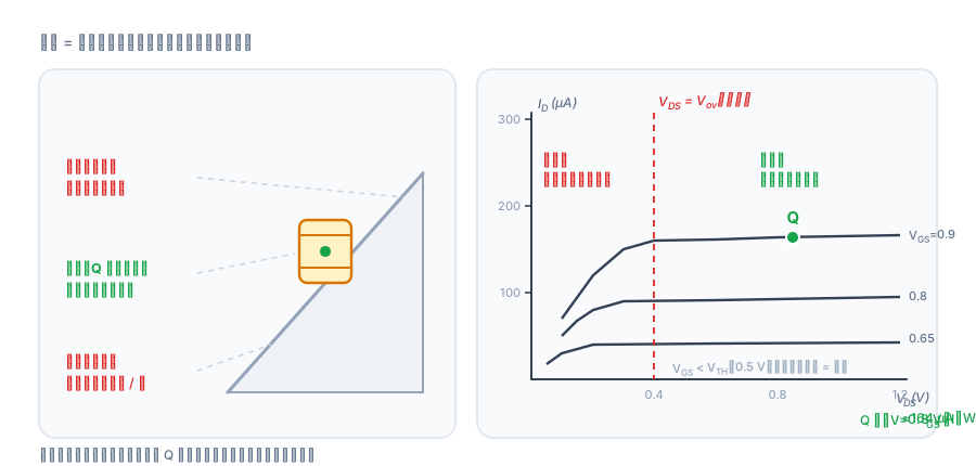
Figure 1: the left side is "why it must sit mid-slope," and the right side is the same thing in datasheet form. The three curves correspond to three values; each curve only flattens out after — that flat stretch is the saturation region, and the only place where amplification can happen.
First, translate "bias" into three sentences
The bias circuit doesn't amplify the signal; it does exactly one thing: give the transistor an accurate, stable standby state. To be "accurate," three conditions must hold:
- Accurate gate voltage: must make the transistor draw exactly the designed standby current ;
- Enough headroom: must leave at least , or the transistor slides into the linear region (the barrel hits bottom);
- Disturbance tolerance: when supply ripple, temperature drift, or process variation come in, this point must not wander.
The first two are solved by calculation; the third is the real craft. Three sentences, three equations:
The third one says: the larger the current and the smaller the overdrive, the larger the transconductance (the stronger the amplification). And also determines "how much the current wobbles when the gate voltage wobbles." Differentiate the first equation and you get the most useful line in this whole article:
When the gate voltage wobbles 1% relative, the current wobbles 2%. That's why the bias voltage must be stable — it gets amplified by the square.
Parameters used throughout the article: , , (), . The bias-branch current is set to 10 µA (power-efficient and sufficient; any smaller and it's drowned out by mismatch and leakage); only the first-generation "quick-and-dirty" example uses 160 µA, to expose the problem.
Generation 1: two bamboo poles carry a barrel (resistive divider)
The most intuitive approach: two resistors divide the voltage, and the midpoint is .
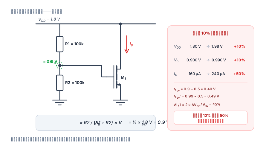
Figure 2: , so is exactly half the supply.
It looks fine, but push it into the numbers and it falls apart. , , :
Now the supply rises 10% (1.80 → 1.98 V):
Supply wobbles 10%, current wobbles 50%. Check it against the square-law expression: — it checks out. The divider doesn't "filter" the noise at all; it just copies the supply fluctuation over unchanged by the divider ratio, and the rest of the amplification is done by the transistor itself.
There are also two minor flaws: the divider itself quietly drinks (larger than some bias currents), and any error in the ratio of the two resistors goes straight into .
Generation 2: swap the lower arm for a "small stone" (diode-connected)
Once you see one key point, the later generations all fall into place. Look at this expression:
For the supply fluctuation to "leak through" to the bias point, how much gets through depends only on the impedance ratio of the upper and lower arms. So there are only two paths: make the lower arm smaller, or make the upper arm bigger.
Replace with a diode-connected MOS (gate tied to drain); its small-signal impedance is only — a big step down from a resistor of tens of kΩ:
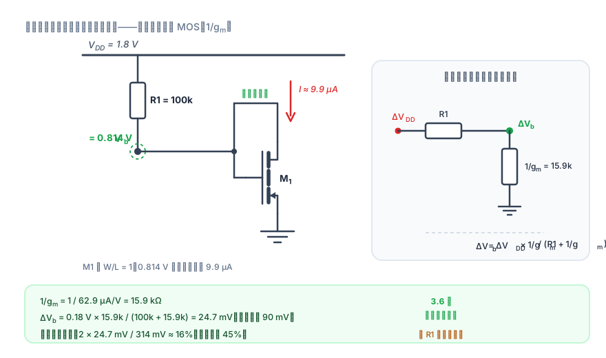
Figure 3: the same "divider" framework, only the lower arm went from 100 kΩ to 15.9 kΩ.
Plug in: ; generation 1 was 90 mV, so it's 3.6× smaller; converted to downstream current wobble, it drops from 45% to about 16%.
This generation also brings a bonus: now automatically tracks the process. When the transistor's threshold runs high, its also runs high, pulling the current back a bit — this is called "self-compensation."
But don't celebrate too early — this road hits a wall at the end: cannot be infinite. is already small, and the remaining fluctuation is almost entirely set by ; and once grows to several MΩ, the on-chip area becomes unmanageable (not to mention parasitic capacitance and noise).
One line to remember this generation: the smaller the lower arm and the larger the upper arm, the less supply noise leaks through.
Generation 3: swap the upper arm for an "invisible bamboo pole" (current source)
Since what we want is an "infinite upper arm," drop the resistor — an ideal current source has infinite internal resistance.
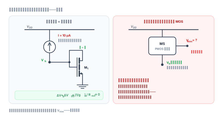
Figure 4: . For an ideal source , the fluctuation is simply divided away; for a real MOS current source , at 10 µA it's about , leaving only 1.4 mV.
Then the problem arises: who supplies the gate voltage for this current source?
It's a PMOS, so it needs a fixed to output a constant current; and that itself needs a stable circuit to generate it. Want "bias independent of the supply"? First you need "current independent of the supply." Want "current independent of the supply"? First you need a "stable gate voltage."
Chicken or egg? Then just — let the circuit give it to itself.
Generation 4: self-biasing — does it work?
Tie the output back to the input to form a closed loop: flows through diode-connected M3 to produce the gate voltage ; M4 copies to get ; then flows through diode-connected M2 to produce , which feeds back to M1's gate.
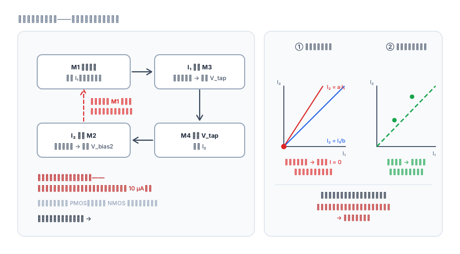
Figure 5: the loop looks beautiful, but write out the equations and there are only two outcomes.
The loop actually has only two constraints, both from the "two transistors sharing one gate voltage" current mirrors:
Substitute:
- (the two mirror ratios are unequal): the only solution is . The whole circuit dies at zero current, with no transistor conducting.
- (the ratios are exactly equal): the equation holds identically, and any value of is "self-consistent." But it never says how much — where the current settles after power-up depends on offset, noise, and the residual charge from the previous moment. The bias is completely indeterminate.
Neither path is usable. Where's the problem? Every element in the loop follows the square law: is a quadratic function of , and is in turn fully determined by — both sides speak the same "language," so neither can pin down the other.
To break the deadlock, the loop must contain an element that doesn't follow the square law.
Generation 5: tuck a stone into the loop (the ΔV/R type)
The cheapest non-linear element is a resistor.
Put it in series with M4's source: the two transistors carry the same current (forced by the 1:1 mirror above), but M4's source is lifted by , so M4 needs a gate-source voltage that is a chunk smaller than M3's. The difference lands exactly on R:
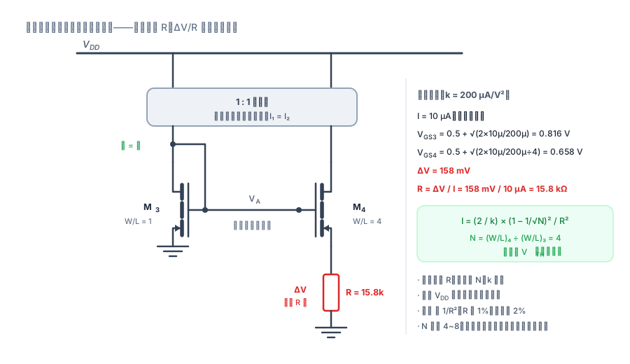
Figure 6: the two transistors have the same gate voltage and the same current but different sizes, so their must differ; the voltage left over can only land on R.
Substitute the square law:
Let and , and solve for the current:
This line is worth staring at for five seconds — every factor tells a story:
- is not in the equation. If the supply rises from 1.8 V to 1.98 V, the current only leaks in a bit through channel-length modulation: . Generation 1 was 50%; here it's 0.9%.
- is subtracted away. The thresholds cancel when the two transistors are subtracted, so this is insensitive to threshold mismatch and temperature drift — its most elegant feature.
- Current . The upside is that can be made large (saving area and improving matching); the downside is the error doubles: if is off by 20%, the current is off by .
- : if mobility is 20% low, the current is 25% high. That leverage stings a bit; in practice it's partially offset by the resistor's temperature drift (polysilicon resistors usually have a positive temperature coefficient, opposite to 's negative one).
Plug in numbers (target 10 µA, ):
Why pick between 4 and 8? If it's too small (say 1.5), is only tens of mV; once mismatch enters, the two transistors are no longer in the same state, and may not even conduct. If it's too large (over 10), M4's overdrive shrinks into the subthreshold region, where the square-law formula itself breaks down. 4–8 is the intersection of "difference large enough" and "still within square law."
But generation 5 only solves half the problem. Remember generation 4's "die at zero current"? is still a solution of this loop: , the equation still holds. So you need a startup circuit — a weak transistor that gives a hard tug at power-up, then turns itself off once the current is established. No ΔV/R circuit exists without a startup circuit.
Generation 6: large currents go V/R
What about large currents like 0.5 mA? Make smaller? First count the cost: with the same , , , we get , , , .
The current is quadratically sensitive to (1% off means 2% wobble); the smaller gets, the harder it is to match, the larger the parasitics, and the resistor stripe still has to be widened — no area is saved at all. So for large currents we simply fall back to the plainest form:
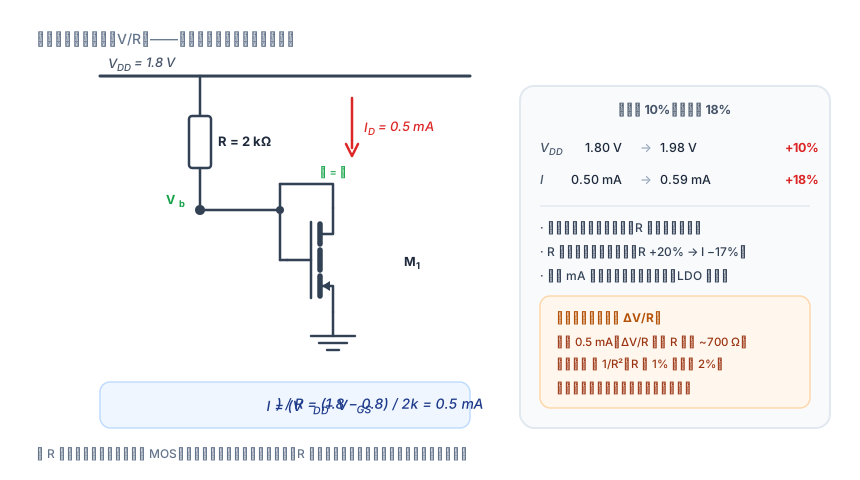
Figure 7: , , and the current is exactly 0.5 mA.
The cost is clear: if rises 10%, the current rises 18% (because the numerator goes from 1.0 V to 1.18 V). So the V/R type only suits situations where the supply is already stable — after an LDO, or in battery-powered designs where accuracy requirements are modest.
Its improved version is the earlier "replace R1 with a current source" figure: replace with a diode-connected MOS (M5), so nodes A and B are nearly shorted, is forced into alignment, and M5 itself stays in saturation. In essence it's still generation 5's "use a transistor as a resistor," just with the current definition moved to a different spot.
Four structures compared side by side
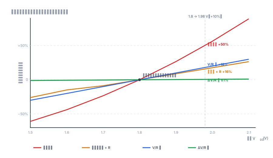
Figure 8: all four curves cross zero at 1.8 V — meaning they're all correct at the nominal point. Whether a circuit's bias is good or not is not judged by its accuracy at the nominal point, but by how fast it runs away after leaving that point.
| Structure | What sets the current | vs. | vs. | vs. error | Best for |
|---|---|---|---|---|---|
| Resistive divider | Divider ratio | Terrible (±10% → ±50%) | No compensation | Only ratio error | Laziest coarse bias, teaching |
| Diode-connected + R | Voltage drop across | Poor (±10% → ±16%) | Self-compensating | First-order (1:1) | Low precision, low voltage, area-saving |
| Current source + diode | The current source | Very good (<1%) | Self-compensating | Good | When a reliable reference current exists |
| ΔV/R type | Very good (≤1%) | Fully cancelled | Second-order (1:2, larger) | Low power, on-chip reference (10–100 µA) | |
| V/R type | Poor (±10% → ±18%) | Self-compensating | First-order | Large currents, regulated supply |
One-line selection guide: for low power plus stability, go ΔV/R; for large current, go V/R; just to set a quick threshold, a resistive divider is enough.
Five easiest pitfalls to step into
1. The zero-current degenerate point (the deadliest)
Closed-loop biasing (generations 4 and 5) both have as a solution. In simulation, a good initial condition via .ic will converge; on silicon, power-up starts from zero — the circuit will quietly lie at zero current, looking perfectly normal, simply not working. A startup circuit is mandatory, and you must verify "slow ramp, fast ramp, and repeated power cycling" all bring it up.
2. Channel-length modulation eats the precision Every derivation in the formulas ignores . In reality, different means the current differs by . At 10 µA, looks large, but if the two branches' differ by 0.2 V, that's a 1% current error — the same order as the entire bias precision target. If you need more accuracy, use a cascode or simply lengthen ().
3. Resistor matching matters more than the value The current only recognizes "how many unit resistors," not how many kΩ you wrote down. So: cut from the same resistor stripe, place in the same orientation, add dummies on both sides, and keep away from power devices and pads. Be especially careful with structures — every bit of resistor error gets doubled.
4. Headroom is a hard budget How many layers can you stack in 1.8 V? Every stacked transistor eats one . Squeeze down to 100 mV to save current, and the transistor can indeed still saturate — but drops, mismatch grows, and speed slows. Current, headroom, speed, precision — you can only pick three of the four.
5. The "ideal current source" is just a symbol on the schematic Built for real, it's . Want a larger ? Add a cascode, at the price of eating another — that's why bias circuits are forever fighting between "saving current" and "saving voltage headroom."
A one-screen cheat sheet
Mnemonics: Keep the barrel mid-slope (the Q point); To resist supply noise, change the impedance ratio, not the divider ratio; To self-bias, the loop must contain an element that doesn't follow the square law; To beat the supply, make disappear from the equation; Finally, never forget: every closed loop needs a startup circuit.
Closing thoughts
The bias circuit is the "least circuit-like" part of analog design: it doesn't amplify, filter, or drive anything — it just quietly puts every transistor in the spot where it should stand. But if it's off, the entire chain is off.
If you came from discrete BJTs, that classic "divider + emitter resistor" bias is actually the same idea as generation 5 here — use a resistor to "measure" the current, and use negative feedback to hold the operating point. The only difference is that in discrete circuits the "feedback" is done by , while on-chip it's done by current mirrors and a source resistor. To hand-calculate a version, you can use the site's BJT divider-bias calculator: enter and target , and it will compute ///, the actual operating point, gain, and input/output impedance — and it will also warn you about classic pitfalls like "divider current is less than 5×."
Next I plan to pull out the "bandgap reference" for its own article — the destination of all bias circuits: how a voltage that barely depends on supply, temperature, or process is assembled from one plus one .